Site menu:

Distribution-free Modeling with cNORM - Mathematical Derivation
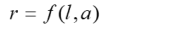
In our mathematical approach, the raw score r of a test scale is modeled as a continuous function of the latent person parameter l and an explanatory variable a.
Parameters
The person parameter l represents an individual's location relative to others in the reference group. The reference group consists of all individuals in the reference population who have the same level of the explanatory variable a. For instance, in an intelligence test designed for use in the USA, the reference group would include all children in the USA of the same age. The location l can be expressed as a rank (percentile) or as a standardized norm score. Since the true location is initially unknown, distribution-free modeling in cNORM begins by forming conventional groups (e.g., age groups). The location is initially estimated using an inverse normal transformation of the respective percentile within the group.
The use of standardized norm scores is based on the implicit assumption that the latent person parameter is normally distributed in the population. This applies to many, but not all, psychological or physiological parameters. For example, a physiological parameter such as the body mass index typically has a positively skewed distribution. Such quantities can nevertheless be modeled effectively using the distribution-free cNORM approach. However, for measures like the body mass index, the resulting norm scores should be reconverted to percentiles at the end of the norming procedure.
The explanatory variable a is a variable that systematically covaries with the quantity or ability being measured. For example, absolute reasoning ability increases monotonically during childhood and adolescence. In this case, the explanatory variable would be age. Other abilities or achievements may depend more on the duration of a child's schooling, in which case the explanatory variable would be the duration of schooling. Theoretically, dichotomous variables (e.g., sex) can also be used as explanatory variables.
Mathematical derivation
Although raw scores are integers in most psychometric tests, for the mathematical derivation a continuum must be assigned to these discrete scores. In this case, the considered function is smooth throughout the measurement range of the test, i.e., the function can usually be differentiated any number of times. Such functions can at any point P(l0, a0) be written as so-called Taylor series:
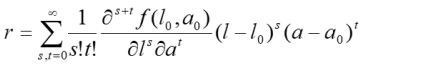
Taylor series typically converge only within a finite radius around the point P for the function being modeled. In practice, however, it has been shown that many functions (e.g., data from psychological or physiological tests) can be approximated extremely well over a sufficient range.
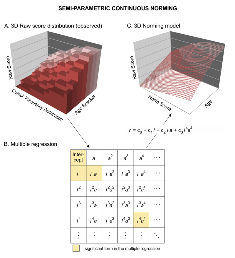
Since the Taylor polynomial represents an infinite sum, this sum can only converge to a finite value if the individual summands become very small rapidly with increasing s and t. This also implies that at large s and t, the summands contribute minimally to the function value. Therefore, the original function can be approximated with sufficient accuracy even if the sum is only calculated up to an index k instead of infinity. This index k serves as a smoothing factor. The higher k is, the more likely it is that noise in the standardization sample will be reflected in the model. To avoid over-fitting, it's recommended not to select k higher than 5. As a rule of thumb, k = 4 will typically lead to a very good approximation. Depending on the age progression, it may also be beneficial to choose slightly higher powers for s than for t (e.g., s = 5 and t = 3).
This approximation ultimately leads to a finite Taylor polynomial, which can be simplified further. The factorials of s and t, as well as the partial derivatives of the function with respect to l and a at point P(l0, a0) are constants, just like l0 and a0. Multiplying the brackets therefore leads to the considerably simplified polynomial:
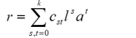
The constants cst of this polynimial can be fitted by multiple regression on the basis of the manifest raw data to estimte a hyperplane:
 |
back to distribution-free modeling |