Site menu:

cNORM - Data Preparation
Content
- Representativeness of the Data Base
- Weighting to Compensate for Violations of Represantativeness
- Determining the Size of the Normative Sample
- Data Preparation in R
Representativeness of the Data Base
The starting point for standardization should always be a representative sample. Establishing representativeness is one of the most difficult tasks of test construction and must therefore be carried out with appropriate care. First of all, it is important to identify those variables that systematically covary with the variable to be measured. In the case of school achievement and intelligence tests, these are, for example, educational background of the parents, the federal state, the socio-economic background, etc. Caution: Increasing the sample size is only beneficial for the quality of the standardization if the covariates do not remain systematically distorted. For example, it would be useless or even counterproductive to increase the size of the sample if the sample was only collected from a single type of school or only in a single region. One advantage of continuous norming is the generally low sample size required. One way of achieving representativeness is therefore to delete as many randomly selected cases from overrepresented strata as necessary, until the individual strata are represented with the required percentage in the overall sample. However, this means that laboriously collected data is lost again.
Weighting to Compensate for Violations of Represantativeness
If representativeness cannot be achieved by removing cases, a second option is to weight the data using Iterative Proportional Fitting (Raking). In simulation studies (Gary et al., 2023, 204), we were able to show that weighting usually leads to more precise norm scores. However, we have so far only conducted these simulation studies using the distribution-free continuous norming method implemented in cNORM. Problems with weighting only arose when the variance in the standardization sample differed greatly from the actual variance in the reference population. Therefore, when applying weighting, make sure that no excessive deviations from representativeness must be compensated for and that subgroups whose average test scores deviate relatively strongly from the population mean are already sufficiently taken into account during data collection.
Determining the Size of the Normative Sample
The appropriate sample size cannot be quantified in a definitive way, but depends on how well the test (or scale) must differentiate in the extreme sections of the norm scale. In many countries, for example, it is common (although not always reasonable) to differentiate between IQ < 70 and IQ > 70 to diagnose developmental disabilities and to choose the appropriate school type or educational track. An IQ test used for school placement must therefore be able to identify a deviation of 2 SDs or more from the population mean as reliably as possible. If, on the other hand, the diagnosis of a reading/spelling disorder is required, a deviation of 1.5 SD from the population mean is generally sufficient for the diagnosis according to DSM-5. As a rule of thumb for determining the ideal sample size, it can be stated that the measurement error caused by the norming procedure is particularly high in those performance areas that are only represented with low probability in the norming sample. (This does not only apply to continuous norming, but to all norming methods.) For example, in a representative random sample of N = 100, the probability that there is no single child with an IQ below 70 is about 10%. For a sample size of N = 200, this probability decreases to 1 %. Doubling the sample size thus notably improves the reliability of the norm score in ranges markedly deviating from the scale mean.
Since continuous norming models are always based on the entire sample, the statistical power of the norming procedure increases for each individual age. As a result, the required size of the norm sample can be substantially reduced. With a sample size of n = 100 per cohort or grade level, the norms already achieve a goodness of fit that is only achieved with conventional norming with sample sizes of n = 400 and more (W. Lenhard & Lenhard, 2021). Thus, not only do the norm scores become more precise, but the standardization projects become more cost-effective overall.
Data Preparation in R
Once a representative sample of sufficient size has been created, the data must be loaded into the R workspace. cNORM excludes cases with missings in relevant variables. For continuous norming, in addition to the variable with the raw scores, an explanatory variable (e.g. age or duration of schooling) is required, which can be represented as a discrete grouping variable or as a continuous variable. Please ensure that the discrete grouping variable is a numerical variable with the group mean of the corresponding continuous variable being used as the variable's value, e.g. 10.5 for all children aged between 10 and 11. If only a continuous variable is initially available when applying the distribution-free method (i.e., modeling with Taylor polynomials), then this variable must be recoded into a discrete grouping variable. However, the method is relatively robust to changes in the granularity of the group subdivision. For example, the modeling result barely depends on whether the sample is devided into age brackets of 6 months or 12 months (see A. Lenhard, Lenhard, Suggate, & Segerer, 2016). The more the course of the raw scores across the explanatory variable deviates from a linear development, the finer the groups should be formed. In parametric modeling with the beta-binomial distribution, an additional group variable is generally unnecessary.
For recoding a continuous explanatory variable into a group variable, the following function can be used:
# Creates a grouping variable for the variable 'age'
# of the ppvt data set. In this example, 12 equidistant
# subgroups are generated.
group <- getGroups(ppvt$age, 12)
When using RStudio, data can easily be imported from other statistical environments using the import function:

For demostration purposes, cNORM includes a cleaned data set from a German test standardization (ELFE 1-6, W. Lenhard & Schneider, 2006, subtest sentence comprehension) that will be used for demonstrating the method. Another large (but unrepresentative) data set for demonstration purposes stems from the adaption of a vocabulary test to the German language (PPVT-4, A. Lenhard, Lenhard, Segerer & Suggate, 2015). In addition, cNORM contains a large data set from the CDC with physiological and biometric data (height, weight and BMI) from over 45,000 children and adolescents between the ages of 2 and 25 from the USA (CDC, 2012). You can retrieve information on the data by typing ?elfe, ?ppvt and ?CDC:
# Loads the cNORM package
library(cNORM)
# Displays the description of the elfe dataset
?elfe
# Displays the first lines of the elfe dataset
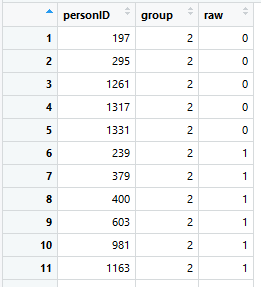
head(elfe)
As you can see, there is no age variable in the 'elfe' data set, only a person ID, a raw score and a grouping variable. In this case, the grouping variable also serves as the continuous explanatory variable, since children were only examined at the very beginning and in the exact middle of the school year during the test standardization. For example, a value of 2.0 means that the children were at the beginning of the second school year, the value 2.5 means that the children were examined in the middle of the second school year. Another possibility would have been to examine children throughout the entire school year. In this case, the duration of schooling (e.g., in weeks) would have to be entered as a continuous explanatory variable. To build the grouping variable, the first and second half of each school year could, for exampe, be aggregated into one group respectively.
In the 'elfe' data set there are seven groups with 200 cases each, i.e. a total of 1400 cases:
# Display descriptive results
by(elfe$raw, elfe$group, summary)
 |
Installation |
Weighting |
 |